# Creating a Graph
Described in the chapter "First steps"
# Configure Graphs
One of the most important graphical objects in TISGraph is the graph. The purpose of graphs is the visualisation of data in the shape of a two-dimensional mapping involving an abscissa and one ore more ordinates.
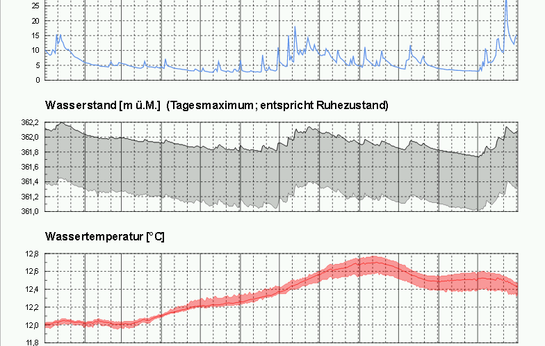
# Legend
Graphs can optionally contain a legend which is automatically based on the graph's data sets. An example would be the following screenshot:
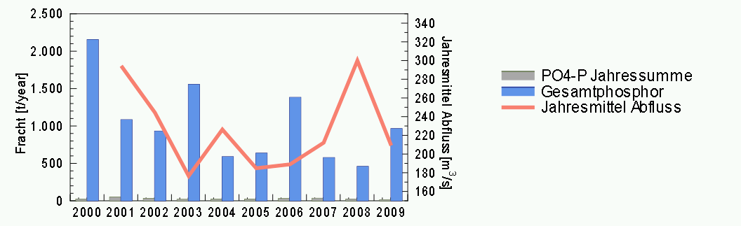
In the edit dialog of a graph, inside Legend tab, properties of the legend such as font style, header and position can be changed. Additionally, you can configure if the legend is supposed to be structured into multiple columns (in case there are a lot of entries).
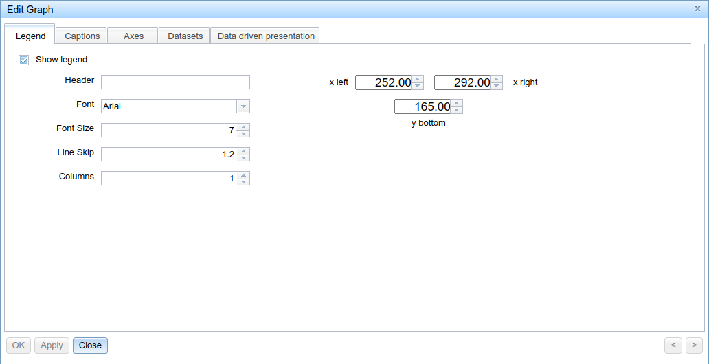
Which datasets are denoted in the legend can be changed in the Datasets tab. It's also possible to add maximum and minimum markers.
# Captions
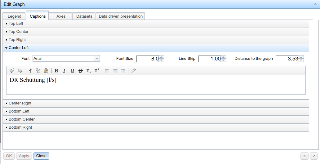
Under the Captions tab, it is possible to configure the text elements next to the graph, for a total of eight different positions. There is a richtext editor available for each of them:
TIP
You can also use text object placeholders for captions. In den Beschriftungen können auch Platzhalter in Textobjekten verwendet werden.
# Axes
In this tab, the appearance and functionality of the different axes can be configured. First in the list is always the abscissa, with one or more ordinates following afterwards.
# Abscissa
The abscissa is usually (but not necessarily) a time-based axis, in which case the X-axis values of incoming data are interpreted as UTC Timestamps for the configured time zone. The time range of the axis is determined either by the document's currently active observation range, or by explicitly setting it in the form of a minimum and maximum in this dialog.
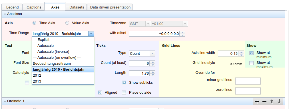
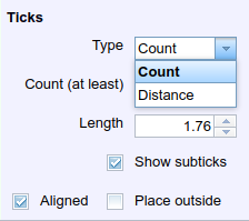
Ticks configuration determines, how the time period is segmented in the graphic. If Count is chosen, the entered value represents the minimum amount of ticks on the axis.
If Distance is chosen instead, then ticks are being set according to the specified time interval, e.g. every 5 years. The format for the time input field is y:M:d h:s:m. If "Aligned" is set, interval borders are kept even when changing the observation period, i.e. in the case of a 5-year interval, ticks are always placed at years 2000, 2005, 2010 etc. If deactivated, ticks on the axis are rearranged accordingly upon changing to a different observation period.

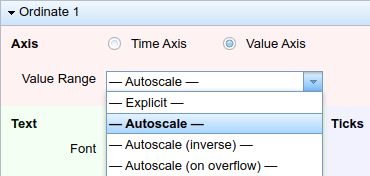
# Ordinates
For ordinates, incoming values are usually interpreted as numerical values. Multiple options are available for determining an ordinate's value range:
- Explicit: Enter a static range explicitly
- Autoscale: automatically scale the range to incoming data points (min, max)
- Autoscale (inverse): does the same, but inverses the minimum and maximum on the axis. I.e., a value range of -25.3 - 34.2 becomes 34.2 - -23.3
- Autoscale (on overflow)*: will default to the explicitly entered range, but will extend it if the maximum is exceeded.
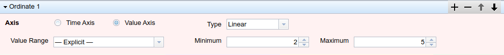
Multiple ordinates may be configured for the same graph, either at the maximum or minimum of the abscissa depending on what is configured in the Show section.
# Datasets
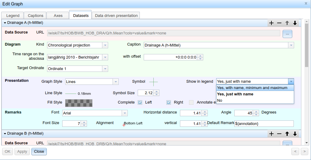
In the Datasets tab, you can configure the data sets to be depicted in the graph. A data set corresponds to an instruction to depict data from a specified source in the specified manner. This tab has four tabs:
- Data Source
- Diagram
- Presentation
- Remarks
Which data is displayed in the end is determined by
- the data source itself
- The "Time range on the abscissa" which can be found in the "Diagram" section.
Data sources are typically provided alongside methods for data access via a TISGraph Data URL, by one of the TISGraph adapters.
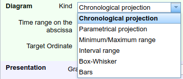
The "Kind" dropdown in the "Diagram" section which type of projection, and therefore which mathematical concept is the basis for the data output. Notably, this determines what kind of data is being expected from the source.
Right below that is the drop down for the abscissa's time range. A time range either be based on an observation range or on explicitly in this dialog specified values for minimum, maximum and time zone. Generally, but not necessarily, the here specified time range corresponds to the abscissa's time range. If the time range is based on the observation period, an offset can be specified to be applied to the range in the graph.
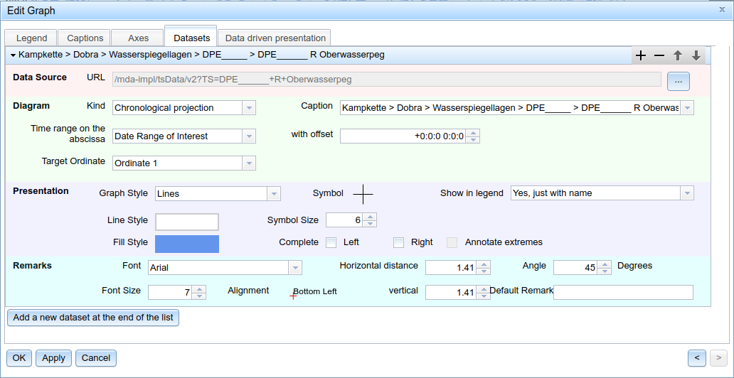
The "Presentation" section serves to configure the precise appearance of the dataset in question, including whether or not it should be included in the legend.
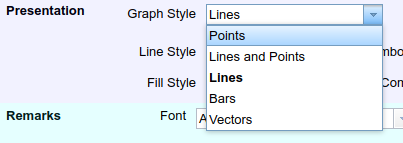
The most common projection type is likely *Chronological projection. Meaning, each timestamp corresponds to a single value. Depending on the desired appearance in the graph, one of the following appearances can be used:
- Points: The selected symbol is being inserted on the location of each data point. The selected color is being used for the inside of said symbol.
- Lines and Points: In addition to points, lines are drawn to link them. You can set the desired color and stroke style.
- Lines: Lines are still being drawn, but data points are not marked by a symbol.
- Bars: Each data point is denoted by a bar of the specified color.
The "Remarks" section allows configuration of optional textual remarks which are added to every data point. You can define both font type and size, as well as where to position it relative to the data point. The input in the "default remark" field can include variables in order to, for instance, denote the value of each point right next to it.
TIP
More detailed information on how to use time stamps and data points in remarks and annotations for different projection types can be found in the chapter for data annotations.